Marketing Attribution Modelling: State of the Art in 2026

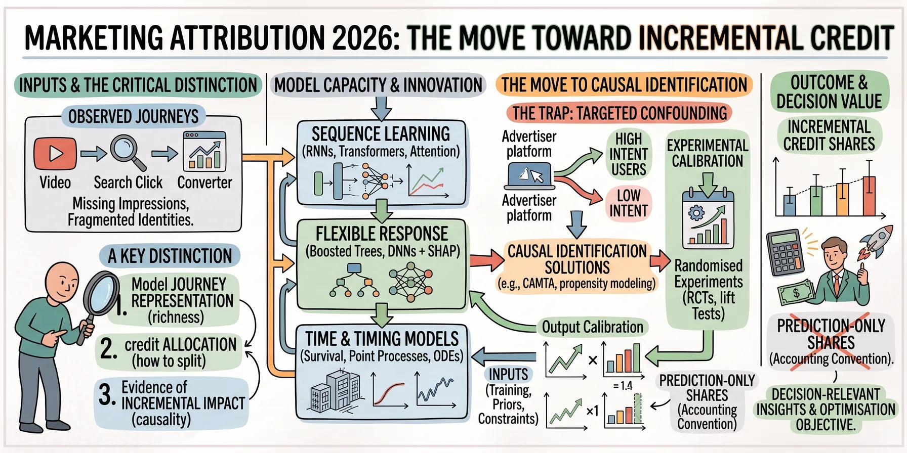
Marketing attribution modelling has recently developed in several directions since Markov chains, Shapley values, and early recurrent neural networks became familiar tools. Models can represent richer customer journeys, handle irregular timing, and attempt to separate advertising effects from targeting decisions. Experimental evidence can now inform attribution systems at scale. Yet there is no universally accepted successor to the older methods, and a more sophisticated conversion model does not automatically produce more credible conversion credit.

Understanding the current landscape requires distinguishing three things:

1. how a model represents a journey,
2. how it distributes credit,
3. and what evidence supports interpreting that credit as incremental impact.

Progress on one does not guarantee progress on the others.

Attribution’s place in modern measurement

Attribution increasingly sits within a measurement programme combining customer-level analysis, marketing mix modelling (MMM), and experiments. These approaches offer different coverage, granularity, and opportunities for causal identification. Attribution provides detailed feedback on observed journeys; MMM can connect aggregate business outcomes with media and other drivers; experiments test specified interventions. Meta’s Building a suite of truth advocates this complementary approach. The IPA’s Making Effectiveness Work adds a useful qualification: choose methods around the business question, rather than assuming that “triangulating” three outputs necessarily creates a better answer.

MMM’s resurgence partly reflects constraints on individual-level tracking and the attraction of methods that work with aggregate data. More accessible tooling has also helped; the Robyn authors explicitly position their open-source package in this context. MMM still faces confounding, correlated spending, and limited identifying variation (see e.g. the Robyn methodology paper). Experiments can strengthen its evidence, just as they can strengthen attribution. This article focuses on attribution itself: what its methods estimate, how they have evolved, and where their outputs deserve confidence.

Prediction, allocation, and causation

Consider a customer who sees a video ad, later clicks a paid-search result, receives a retargeting impression, and purchases. Several legitimate questions can be asked about this sequence.

A prediction model asks how likely the customer is to purchase, given the recorded history. An allocation method asks how to divide credit among the touches. A causal model asks how the outcome would change under an intervention: suppressing the video campaign, removing retargeting eligibility, or changing the advertising policy.

Those questions need different evidence. Retargeting might strongly predict a purchase because it reaches people already close to buying. Its predictive contribution could therefore exceed its incremental effect. Conversely, an early video exposure might initiate interest that later appears as branded search. A model that conditions on that search without considering its role in the causal pathway can obscure the earlier influence.

There is also a baseline question. Are we distributing one observed purchase, explaining a predicted probability relative to a reference population, or allocating an estimated increase above a no-advertising outcome? All can generate fractional numbers labelled “attribution”, but the numbers have different meanings.

This distinction is especially important when normalising credits to 100%. Allocating every purchase completely among recorded marketing touches is an accounting convention. It does not demonstrate that advertising caused every purchase. A system intended to estimate incremental outcomes needs an explicit treatment of the baseline and a clear explanation of any subsequent normalisation.

Markov and Shapley remain useful foundations

Markov attribution represents journeys as transitions between states, often channels, with conversion and non-conversion endpoints. Removal-based methods assess how the model’s conversion probability changes when a channel is removed according to a specified rule, then translate those changes into credit.

The familiar first-order version conditions the next transition on the current state. Higher-order versions retain more history: the original graph-based attribution literature already considered both. It is therefore inaccurate to say that Markov models fundamentally cannot capture sequence context. The practical trade-off is between richer states and sufficient observations to estimate their transitions. Anderl et al., 2016

The deeper issue is what removal means. If the video touch disappears, does the customer still search? Is the path terminated, rerouted, or otherwise reconstructed? These choices define the modelled comparison. A removal effect becomes a causal effect only with additional justification connecting the altered model to an actual intervention.

Shapley attribution addresses a different component: allocating the value of a coalition among its members by averaging marginal contributions across possible coalition contexts. The members might be channels or individual touches; the value might be predicted conversion probability, revenue, or an estimated causal outcome.

Consequently, “Shapley versus neural networks” is often the wrong comparison. A neural network can supply the value function that Shapley allocates. DeepMTA, for example, combines a phased-LSTM conversion model with additive, Shapley-based feature attribution. It is a concrete bridge between deep sequence modelling and game-theoretic allocation. DeepMTA, 2020

Shapley’s allocation properties do not determine whether the underlying value function is correct. Practical decisions remain: what counts as a player, how absent touches are represented, whether chronological order is preserved, and which baseline is used. Exact calculation can be expensive, but sampling and model-specific algorithms make the computational story more nuanced than “Shapley is exponential, attention is linear”.

Flexible response models and feature attribution

One broadly accessible approach is to predict conversion or revenue using logistic regression, boosted trees, or neural networks, then derive contributions through feature ablation, gradients, or SHAP. SHAP provides a framework for assigning feature contributions to a model output relative to a baseline. Its immediate object is the prediction being explained. Lundberg and Lee, 2017

This approach separates two design decisions: choosing a response model and choosing an explanation method. An analyst can improve predictive calibration, add nonlinear interactions, and test alternative credit rules without rebuilding the entire pipeline.

However, the representation constrains the explanation. A table containing channel exposure counts and recency cannot recover every detail of exposure order. Explaining a feature such as “number of search clicks” is different from valuing a particular click. Grouping feature contributions into channel totals requires care when channels have multiple correlated features.

Ablation also needs a plausible reference. Setting search clicks to zero while retaining downstream behaviour that depended on those clicks can create an unrealistic customer. Replacing missing features with background values defines another comparison, with its own assumptions. These pipelines can provide useful descriptive attribution and strong benchmarks, but their convenience does not establish causal validity — or prove that they dominate commercial practice.

Sequence learning: RNNs, attention, and Transformers

Recurrent architectures such as LSTMs and GRUs update an internal representation as touches arrive. They can learn that the same exposure has different predictive relevance depending on previous interactions, elapsed time, frequency, and customer characteristics. They replace manually specified history states with learned representations, although their capacity still depends on training data and design choices.

Attention adds a mechanism for weighting information from different parts of the sequence. DARNN, introduced in 2018, uses dual attention and incorporates pre-conversion click behaviour alongside exposure information. DNAMTA, also from 2018, combines attention-based modelling with user context. These papers establish that attention-based attribution has a substantial history; it is not a development that began with the recent popularity of large language models.

An attention mechanism can yield convenient touchpoint weights during inference. But convenience is not validation. Attention weights can differ from other measures of a feature’s influence on the prediction. Research on attention explanations has demonstrated this problem and proposed tests for assessing when interpretation is justified. Those studies concern model explanations; interpreting attention as advertising causation requires further evidence still. Jain and Wallace, 2019, Wiegreffe and Pinter, 2019

Transformers provide another way to learn relationships across a journey through attention, with explicit representations of order and potentially elapsed time. They can incorporate campaign and customer embeddings and contextual features. The benefit is flexible representation; the cost includes data requirements and computational complexity. Standard full self-attention scales quadratically with sequence length, although implementations and variants can change that trade-off.

LinkedIn’s LiDDA is a documented industrial example. First submitted in 2025 and revised in May 2026, its paper describes a Transformer-based system developed for LinkedIn’s own marketing and extended to advertising applications. It uses timing information and contextual embeddings, converts attention into relative path credits, and calibrates against aggregate estimates. The paper also describes probabilistic handling of missing impressions and training-time calibration to MMM outputs. These are disclosed components of a deployed system, rather than evidence that Transformers universally outperform other attribution methods.

The methodological question remains unchanged across architectures: how are learned representations converted into credit, and how is that credit checked? A Transformer can improve the first part of that process without settling the second.

Time matters beyond sequence order

A customer seeing three ads within ten minutes is different from one seeing them over three weeks. Ordering alone does not capture elapsed time, and a fixed attribution window can conceal important differences in delay and persistence.

Survival and hazard models address the timing of conversion. Temporal point processes model when events occur and how previous events change subsequent event intensity. These families are useful when the goal includes distinguishing a direct association with conversion from pathways operating through later touches.

A graphical point-process framework proposed by Tao and colleagues explicitly models relationships among touchpoint types and derives two forms of removal effect for path-level attribution. Its contribution is a more structured account of how removing a touch changes the modelled process, including its relationships with subsequent activity. The causal interpretation still depends on the assumptions connecting that process to the real world. Graphical point-process attribution, 2023

Neural differential-equation models extend the representation of time in another direction. A 2024 workshop paper explores an ODE-LSTM with attention for irregularly sampled customer journeys. Its results discuss both benefits and limitations, including differences between predictive and attribution-oriented evaluation. It is an example of an emerging modelling option, rather than an established replacement for other sequence methods.

These approaches make an important point about progress: better attribution research is not simply a succession of larger architectures. Explicitly representing time, censoring, and pathways between events can matter as much as additional model capacity.

Causal MTA: learning under targeted exposure

Advertising histories are selected rather than randomly assigned. Platforms use information about intent, interests, and prior behaviour to decide who sees an ad. Earlier advertising may also change those characteristics, affecting both later exposure and eventual conversion. This makes causal attribution a longitudinal problem, not just a prediction problem with a few extra control variables.

Research labelled causal MTA attempts to address this selection. CAMTA combines recurrent modelling with a mechanism intended to reduce bias in channel assignment over time. CausalMTA explicitly considers confounding from static and dynamic user preferences and the resulting difficulty of predicting counterfactual journeys. DCRMTA investigates learning representations that retain useful user information while attempting to remove confounding. These represent different research proposals, not a single standard algorithm.

The broader toolkit includes modelling exposure propensities, reweighting observations, balancing representations, and explicitly specifying how treatments and outcomes evolve. Each requires a credible identification argument. Adjustment cannot recover information that the data never contain merely because the adjustment model is flexible.

For example, if high-intent customers almost always receive retargeting, there may be little comparable evidence about what happens without it. This is an overlap problem. If important intent signals are unavailable, adjustment for recorded variables may leave confounding. If later clicks are consequences of an earlier ad, treating them as ordinary baseline controls can alter the effect being estimated.

A paper’s improved conversion AUC does not resolve these problems. Nor does an attribution pattern that looks intuitively reasonable. Large-scale comparisons of observational estimates with advertising experiments have found substantial difficulties recovering experimental effects, even with rich data and sophisticated methods. That evidence concerns advertising-effect estimation more broadly; it should motivate stronger evaluation of MTA, without being misrepresented as a direct test of every attribution architecture. Gordon, Moakler, and Zettelmeyer, 2023

The useful advance is greater explicitness about the causal problem. A method should state its intervention, assumptions, adjustment strategy, and validation evidence. “Causal” in the title is a starting point for inspection.

Experimental calibration: connecting credit to measured lift

Attribution models can incorporate experimental evidence. There is no fundamental incompatibility with Markov models, Shapley allocation, or neural networks. Compatibility depends on where the evidence enters the system and whether the experimental comparison matches the quantity being modelled.

Calibrating outputs

The simplest approach compares attributed outcomes with incremental outcomes from a suitable experiment. If attribution assigns 1,000 conversions to a campaign while a comparable experiment estimates 600 incremental conversions, an illustrative multiplier is 0.6. Applying it aligns the campaign total with the experimental estimate.

Google’s Modern Measurement Playbook describes this approach, including matching the campaigns and measurement period and using the multiplier between experiments. It also discusses comparability, changes in incrementality, and the difficulty of judging relative performance when only some channels have experimental evidence.

Such a multiplier can improve interpretation of a reported total. It cannot establish that every audience, creative, or touchpoint deserves exactly 60% of its previous credit. Within the calibrated group, a uniform multiplier preserves the existing ranking and relative allocation, including any mistakes.

Calibrating the model

Experimental evidence can also enter the model-fitting process. Depending on the implementation, it can supply training observations, informative priors, constraints, or an additional loss penalising disagreement with measured effects. A neural model can, in principle, be trained so that its aggregate predictions under the tested intervention agree with experimental estimates, allowing for uncertainty.

This is a design pattern, not a feature automatically provided by every published model. The analyst must define the intervention inside the model and aggregate predictions over the correct population. For a Shapley pipeline, experiments might inform the response function used to value coalitions. A campaign-level experiment does not identify all coalition values, especially when interactions are important.

An illustrative training objective could combine ordinary predictive fit with a term comparing model-implied lift against experimental lift. The relative weighting should reflect uncertainty and the intended task. Forcing exact agreement with a noisy experiment can replace one error with another; using the same study for calibration and final validation also overstates the independence of the check.

Learning calibration across experiments

A further approach learns a relationship between campaign characteristics, attribution signals, and experimentally measured effects. Predicted Incrementality by Experimentation (PIE) formalises this at campaign level: train on a collection of experiments, then predict incrementality for campaigns without their own experiment. This extends experimental information through modelling; it does not turn untested campaigns into randomised experiments.

Amazon’s 2025 MTA paper describes a concrete extension to touchpoint attribution. Attribution-model outputs become inputs to a causal calibration model trained against campaign-level randomised results. The calibration is then applied to touchpoint signals, which can be aggregated into reporting shares. Amazon describes an ensemble that can combine simpler attribution signals with more flexible model-based ones. Its evidence base must remain representative and current for that learned mapping to remain useful.

Across these approaches, the central limitation is granularity. Matching a campaign’s incremental total does not uniquely determine the contributions of its individual touches. Experimental calibration provides identifying information where the experiment has leverage; finer decomposition still depends on modelling assumptions and allocation choices.

Interactions and the meaning of a total

Consider an illustrative business with 100 conversions without two channels, 120 with channel A alone, 110 with B alone, and 150 with both. The combined incremental effect is 50. Removing A from the combined policy loses 40 conversions; removing B loses 30. Those removal effects sum to 70 because the channels interact.

A Shapley allocation of the 50-conversion gain would give A 30 and B 20, averaging each channel’s contribution when added first and second. That is a coherent allocation convention. It differs from the separate removal effects without contradicting them.

This matters for calibration: an experiment suppressing one channel while another remains active identifies a different contrast from an allocation of the total joint effect. Before asking estimates to agree, check the treatment, population, outcome, horizon, and interaction context. Even excellent experiments do not remove the need to define what attribution is allocating.

Google, Meta, Amazon, LinkedIn: what commercial systems reveal

Public disclosures provide evidence of real implementation, but visibility varies substantially. A technical paper can describe modelling choices without independently validating every reported benefit; a product announcement usually reveals much less.

Google’s data-driven attribution documentation separates conversion-probability modelling from fractional credit assignment. It says that models estimate counterfactual gains of Google ad exposures using training data from randomised trials. This is evidence of experimental information entering the modelling process, rather than merely a later reporting adjustment. It should not be read as proof that every touchpoint on every channel is independently experimentally identified. Google Analytics methodology

The LinkedIn and Amazon systems illustrate different combinations of components. LiDDA joins learned path weights with aggregate calibration; Amazon describes using experimental effects to learn a calibration of attribution signals. Neither is adequately described by a single label such as “attention attribution” or “causal AI”. Their architectures, data sources, calibration targets, and reporting conventions all matter.

Meta’s Incremental Attribution is another significant development. Meta reported completing its global rollout in Q2 2025. Its Building a suite of truth report states that the product uses machine-learning models trained on Conversion Lift data to optimise delivery for incremental conversions, and allows comparison with other attribution reporting. A January 2026 update describes further model development and growing adoption (see e.g. Meta’s Q2 2025 remarks and the January 2026 update).

Its relevance extends beyond assigning a different number to yesterday’s conversions: an incremental objective can change which opportunities the delivery system pursues. Reporting and optimisation must therefore be evaluated separately. Better business outcomes under a bidding policy would support that policy, while accuracy of reported incremental conversions requires a measurement comparison.

Meta’s product also has a different scope from an advertiser-wide, cross-channel MTA model. Public materials explain its intended objective and experimental training source, but do not expose enough detail to equate it with a specific published architecture or establish the correctness of each granular estimate. The defensible claim is that experiment-informed incremental attribution is commercially deployed — not that the individual causal contribution of every conversion has become observable.

Comparing the method families

These categories overlap: a deployed system can combine a sequence model, a Shapley allocation, and an experimental calibration layer.

Family	Main contribution	Experimental support	Evidence and limitation
Markov / removal models	Modelled transitions and removal effects	Output calibration; model selection or custom constraints	Established baseline; removal semantics determine interpretation
Shapley-based allocation	Explicit allocation of a defined value function	Experiments can inform that function or check aggregates	Established framework; allocation properties do not validate the value function
Response model plus explanations	Flexible prediction with modular credit extraction	Training data, aggregate constraints, or output calibration	Practical modelling approach; feature credit needs a marketing interpretation
RNN / attention / Transformer models	Rich sequence and contextual representations	Possible during fitting or after inference; implementation-specific	Research and documented industrial examples; attention is not causal proof
Hazard / point-process / continuous-time models	Timing, evolving intensity, and event pathways	Experimental comparisons or custom fitting constraints	Established statistical families with newer attribution research variants
Observational causal MTA	Explicit adjustment for exposure selection	Experiments can test or strengthen identifying assumptions	Active research; overlap and unobserved confounding remain central
Experiment-trained calibration systems	Mapping granular signals toward experimental effects	Experiments are part of the system’s evidence base	Documented industrial implementation; granular decomposition and transport remain model-dependent

How to assess a state-of-the-art claim

A useful assessment separates predictive performance, allocation behaviour, causal validity, and decision value. No single benchmark establishes all four.

For prediction, inspect held-out discrimination and probability calibration, with time-based splits where appropriate. Guard against leakage from information unavailable at the intended scoring time. For allocation, examine sensitivity to random seeds, retraining periods, baselines, channel grouping, and journey truncation. A stable prediction can coexist with unstable credit.

For causal validity, ask what ground truth the evaluation actually supplies. Synthetic data can test recovery under a known generating process, but only within that simulated world. Removing model inputs tests behaviour under perturbation; it is not equivalent to withholding ads from people. Offline budget replay depends on assumptions about outcomes under unobserved delivery decisions. Independent experiments provide stronger evidence about their tested interventions, while still having uncertainty and limited scope.

Data coverage deserves equal attention. Missing impressions, fragmented identities, and consent-related selection can change which journeys enter training. Imputing touches adds assumptions; it does not restore observed truth. Conversion windows and delayed outcomes create further choices about censoring and the population considered non-converting. Analyse how these choices affect channel credit, rather than treating them as preprocessing details.

Finally, test the decision the attribution will support. Descriptive credit for past activity is not automatically an estimate of the return on the next unit of spend. Saturation, auction conditions, targeting changes, and interactions can alter marginal returns. A useful operational model should be evaluated under the policy changes it encourages, with uncertainty visible at the level where decisions are made.

What a marketing analyst should take away

The current frontier is best understood as a combination of better journey representations, clearer causal targets, and stronger links to experimental evidence. Each can improve an attribution system, but their benefits should be demonstrated separately.

Start by defining the output: observed-conversion shares, predictive contributions, incremental outcomes, or a signal for optimisation. Specify the baseline and intervention before selecting the architecture. Build credible simpler benchmarks, then add sequence or timing complexity where the data and evaluation justify it.

Where experiments are available, use them deliberately: to validate, select, calibrate, or train models. Explain which role they play and reserve independent evidence for assessment where possible. Preserve the distinction between an experimentally supported aggregate and a model-dependent distribution of that aggregate across touches.

For commercial products, ask for the same information expected from an internal model: observable coverage, allocation rules, calibration targets, uncertainty, and validation design. Accept that some details will remain proprietary, and make that limit part of how much confidence the outputs receive.

Shapley, Markov, and LSTMs remain useful reference points. The more consequential question today is how an attribution system connects its granular numbers to a well-defined quantity and credible evidence. That connection is what makes a model useful for measurement — and worth acting on.